Multi-Agent Reinforcement Learning (MARL) is an emerging field which has gained considerable attention in recent times due to the success of the StarCraft II model AlphaStar.
This attention has inspired a higher level of understanding and exploration in this field.
Currently, MARL faces issues of scalability and training methodology that accounts for coordinated behaviour while maintaining real-time decision processes.
This survey covers traditional RL frameworks like Markov Decision Process, Q-Learning, Actor-Critic and policy gradient,
then transitions to recent methods like Multi-Agent Deep Deterministic Policy Gradient with Communication and QMIX architectures.
Lastly the performance of learning agents via the StarCraft Multi-Agent Challenge is examined.
Reinforcement Learning mimics human psychology by maximizing long-term reward when interacting with an environment.
RL has been used to train agents to perform tasks such as physical object manipulation and game playing as well or better than human counterparts.
While RL has been around in some form for many years, the merging of Deep Neural Networks and RL in 2015
helped solve issues of high dimensionality in RL environments and reinvigorated research in the field.
Many complex real world tasks rely on the interactions between multiple participants,
and so the next frontier for Deep RL has been to model cooperation, competition and communication between multiple agents.
This documnent both provides background on traditional RL while focusing on the modern challenges and solutions involved in Multi-Agent Reinforment Learning (MARL).
Multi-agent learning senarios suffer from problems of high-dimensional data, non-stationarity of optimal policies, and partial observability of learning environments.
Many MARL algorithms address these issues by modifying or building upon traditional RL algorithms from Deep Q-Learning and Actor-Critic methods to Policy Gradients.
MARL expands on these base algorithms by adding communication layers, minimax optimization and other tools to allow cooperation or competition between multiple agents.
Sometimes, a single model is used to control a whole swath of agents or conversely each agent has its own, separately trained, model.
While large advances have been made to MARL algorithms in the last few years the inherent complexities of multi-agent environments make
it one the most active areas of study in Machine Learning.
A Markov Decision Process (MDP) provides a mathematical framework for senarios where a single agent makes decisions in an environment to optimize reward, and each
decision has a randomized effect on the environment.
Formally it is defined as a tuple \(\langle S,A,f,p \rangle \), where \(S\) is a finite set of environment states, \(A\) is a finite set of agent actions,
\(f: S \times A \times S \rightarrow [0,1]\) is a state transition function, and \(p: S \times A \times S \rightarrow \mathbb{R}\) is a reward function.
At each time step \(t\), the agent can observe the environment state \(s_t \in S\) and take some action \(a_t \in A\).
The action transitions the environment to state \(s_{t+1}\) with probability \( f(s_t,a_t,s_{t+1}) \) where the agent receives some scalar reward \(r_{t+1} = p(s_t,a_t,s_{t+1}) \).
Neural networks rely on the assumption that data samples are drawn independently and identically from a distribution (iid).
Training a neural network on samples from an episode would not fulfill this requirement as each state is directly correlated with the next state.
To get around this limitation a finite replay buffer is typically used in reinforcement learning problems.
All state-action pairs and their rewards are saved to a replay buffer during an episode.
Once the episode is completed the rewards for this episode can be modified to include the size of rewards obtained later in the episode.
This allows rewards from a given action to reflect how well that action impacted the future, which is paramount in episodes with sparse rewards.
During training, all state-action-reward tuples in the reply buffer are randomly shuffled then fed to the model.
Provided a long episode with sparse rewards it can be difficult to determine which action caused a specific reward.
This problem is known as the credit assignment problem and is another reason a replay buffer is used.
The replay buffer allows for the rewards to be adjusted prior to training.
A target network is a copy of the architecture of the main network used during training.
This target network is updated less often than the main network used in the reinforcement learning task.
This target network may also have different hyperparameters and be bounded in how large of a gradient may be backpropagated at one time.
Periodically the target network is copied to the main network and training continues.
The target network provides stability to the overall reinforcement learning architecture.
It prevents the main network from "falling off of an edge" while training by constraining how much it may change during training.
Model free means the reinforcement learning architecture has no knowledge of the specific problem at hand.
The same architecture can be used on multiple environments and will learn/adapt to each one without significant changes.
Typically, reinforcement learning architectures are build using one (or both) of these two types of functions.
Policy functions directly map a state to an action.
Value functions are given an action and state, and then calculate a score based on how close the given action is to the best action for the provided state.
In many real-world senarios partial observability provides a confounding factor for Reinforcement Learning.
If the entire environment state is not observable to all agents, then the problem must be modelled using a partially observable Markov Game (POMG).
Partial observability can occur if previous state data influences the optimal actions in the current state.
For example, if an agent is trained to play a videogame through still game images, previous images may have an important impact on current state strategy.
In many multi-agent senarios the state-action space is simply too large, so partial observability is imposed to make the problem computationally tractible.
There are two types of learners in reinforcement learning - off policy and on policy learning.
Off policy means the architecture learns regardless of the actions of the agent - ie. Q-Learning.
In Q-learning, the agent is trying to optimize a value function which is unaffected by the action the agent took.
Each action the agent takes will either reinforce what has been learned and reap larger rewards (exploitation) or provide more information about the system (exploration).
Both exploitation and exploration will help to train the value function.
On policy means the architecture learns directly due to the actions of the agent - ie. Policy Gradient Methods.
Policy based methods typically output a probability over which action should be taken.
They inherantly wrap exploration and exploitation together as the best action will be chosen on a probablistic level.
In a MDP, the agent's goal is to maximize expected reward over the time horizon (in this case infinite):
\[R_t = E \left\{ \displaystyle\sum_{i=0}^{\infty} \gamma^i r_{t+i+1} \right\} \]
Where \(\gamma \in \lbrack 0,1) \) is the discount factor and the expectation is taken over the probabilistic state transitions.
The behavior of an agent is determined by its policy \(\pi\), which describes how an agent will choose an action given the current state.
In order to achieve the goal of learning a policy that will maximize long term reward we define the utility function:
Q-Learning is an iterative procedure used to approximate the optimal Q function \(Q^*(s,a) = max_{\pi}Q^{\pi}(s,a)\).
The Q-table stores current estimates of previously explored state, action pairs and is updated using the equation:
Where the \(a'\) are potential agent actions in state \(s_{t+1}\), and \(\alpha \in (0,1]\) is the learning rate.
Since the Q-value updates do not require knowledge about the probabilistic state transition function or the reward function,
Q-Learning is considered model-free.
In order for the sequence of Q-functions described above to converge to the optimal \(Q^*\), the agent must try all actions from all states with non-zero probability.
Therefore the learned policy cannot be the deterministic, prohibiting the greedy policy that picks the action with highest Q-value for every state.
Instead, the policy must be a mapping from an environment state to a probability distribution over the agent actions, which is non-zero for all actions.
This is known as the exploitation-exploration tradeoff, where a policy seeks to exploit actions that are known to be high value while also attempting unexplored actions.
One example of such a policy is \(\epsilon\)-greedy exploration, where the agent chooses a random action with probability \(\epsilon\) and the action with
largest Q-value with probability \((1-\epsilon)\).
Other examples include Boltzmann exploration and entropy sampling.
The state-action space in many environments can be quite large, which can make learning a complete Q-table computationally intractible.
While each of these state-action pairs are unique, some may occur infrequently or may be strategically similar or other pairs.
Deep Q-Learning seeks to generalize the knowledge of explored states by approximating \(Q(s,a)\) with a Deep Q-Network (DQN), \(Q(s,a|\theta)\)
Where \(\theta\) is the weights of a neural network that parametrize the Q-values. The weights are updated by minimizing the loss function:
There are two key components to the above equation that improve convergence.
First is the use of an experience replay buffer \(D\), containing tuples \( (s_j, a_j, r_j, s_{j+1})^J_{j=1}\) that have been observed by the learning agent.
Rather than updating the the Q-network with each new explored state, the network is updated using uniformly drawn samples from the replay buffer.
Second is the target network \(\widehat{Q}\), whose weights are kept fixed for a certain number of iterations and then updated periodically.
Actor-Critic methods are one of the most popular forms of reinforcement learning.
In this scenario there are two networks, an actor and a critic.
The actor network determines what should be the next action taken.
This actor is typically a policy function which learns the best action for a given state.
The critic dictates if the provided action is "good" given the current state.
This critic network is typically a value function that provides a score for how close the given action is to the optimal action.
Most RL problems fall under continuous action spaces. Discretizing a continuous action space often results in the curse of dimensionality,
where the problem becomes computationally intractable due to high dimensionality.
Google DeepMind created Deep Deterministic Policy Gradient (DDPG) which is a policy-gradient actor-critic algorithm that is also off-policy and model-free.
DDPG uses a stochastic behavior policy for good exploration but estimates a deterministic target policy.
A policy gradient algorithm utilizes a form of policy iteration where the policy is evaluated and then the policy gradient is maximized.
As DDPG is a policy gradient algorithm this is used in both determining the deterministic target policy and the behavior policy.
The target policy is the actor and the behavior policy is the critic.
In other words, DDPG concurrently learns a Q-Function (critic) and a policy (actor) by using off-policy data and the Bellman equation to learn the
Q-function and uses the Q-function to learn the policy .
The actor is used to compute action predictions for the current state.
The critic generates a temporal-difference (TD) error signal for each time step based on what it believes is the best action for that timestep resulting in the next timestep.
The input of the actor network is the current state and outputs a single real value representing an action chosen from a continuous action space.
The critic is given the current state and output of the action given by the actor.
The output of the critic is the estimation of the temporal difference of the Q-value and provided action.
Data is not I.I.D as it’s correlated through time, so a replay buffer is used to uncorrelate the training samples.
Directly updating the actor and critic neural networks can lead to instability; thus, target networks are used to stabilize the updates
.
In a discrete action space one can directly search for an optimal action.
In a continuous action space this is a painfully expensive subroutine.
Sadly, the implementation of DDPG does not support parallelization .
However, DDPG is specifically designed for, and can only be used with, continuous action spaces .
This charcteristic of DDPG negates the need for a direct search for an optimal action.
The Q-function is approximated using a gradient-based learning rule for the critic network:
DDPG is performed by minimizing the Mean Square Bellman Equation Loss with stochastic gradient descent:
As the action space is continuous it is assumed that the Q-function is differentiable with respect to the action.
Thus, the Q-function parameters are treated as constants and gradient ascent is used in respect to the policy parameters only:
Lastly, policy gradient based models handle exploration via a probablistic choice of action from the actor.
To enhance exploration uncorrelated and mean-zeroed Gaussian noise is used on the output of the actor network prior to action choice.
That noise is uncorrelated, mean-zero Gaussian noise.
The psudocode for this architecture is shown below:
A Markov Game, also known as a stochastic game, is a natural extension of a MDP to a senario with \(m\) agents.
It is defined by \(\langle S,\mathcal{A},F,P \rangle \) where S remains a finite set of states, \(\mathcal{A}\) = \(A_1 \times ... \times A_m\) is the joint action set, and
\(F: S \times \mathcal{A} \times S \rightarrow [0,1]\) and \(P: S \times \mathcal{A} \times S \rightarrow \mathbb{R}^m\) are the state transition and joint reward functions,
repectively, which both depend on all agent actions.
The simplest solution to extend Deep Q-Learning to the multi-agent case would be to have each agent learn their optimal policy independently.
Each single agent has an autonomous Q-learning algorithm and other agents are considered part of the environment.
However, the interactions of multiple agents can reshape the environment so that the optimal policy may change drastically
throughout the learning process.
This non-stationarity - a shifting of an optimal policy over the time horizon - poses one of largest problems for MARL as
convergence guarantees for Q-learning break down in this context.
Several algorithms have been developed in an attempt to rectify the issue, and some yeild positive experimental results.
Deep Q-Learning with an experience replay buffer was not designed for non-stationary multi-agent environments, but modifications to this framework can help to
improve empirical convergence results.
One example is Deep Repeated Update Q-Learning (DRUQL), which aims to solve the problem of policy-bias in traditional Q-learning.
The Q-value of an action is only updated when that action is executed.
Consequently, the effective learning rate of an action depends on the probability that an action is selected, creating systematic bias towards certain
actions through frequent updates.
If the reward information for all actions were available at every state and at every time step, this problem would not exist; however, that is clearly
not the case as a single action must be chosen.
This problem is distinct from the previously discussed notion of exploitation vs. exploraiton which does not concern learning rates.
In a non-stationary environment this problem is exacerbated because learning is biased towards previously optimal policies which may now be obsolete.
DRUQL stores each state transtion in an experience replay buffer \(D\), but also includes an effective learning rate \(z_{\pi(s_t,a_t)} = 1 - (1-\alpha)^{\frac{1}{\pi(s_t,a_t)}}\)
where \(\pi(s_t,a_t)\) is the probability of selecting action \(a_t\) in state \(s_t\) determined by policy \(\pi\).
When drawing from buffer \(D\) a tuple \( (s_j, a_j, r_j, s_{j+1},z_{\pi(s_{j+1},a_{j+1})} )\) is uniformly selected.
Then during gradient decent vector \(z_i\) is populated with the sampled \(z_{\pi(s,u)}\), and the neural network weights are updated by
\(\theta_{i+1} \leftarrow \theta_i + z_i \nabla_{\theta_i} \mathcal{L}(s_t,a_t|\theta_i) \) where \(\mathcal{L}(s_t,a_t|\theta_i) \) is the loss function from Section 2.9.
The result of this modification to Deep Q-Learning is that the learning rate for high probability actions is reduced in proportion to their frequency so that policy bias
is reduced or eliminated.
Parital observability, as discussed in Section 2.6, provides another problem for Multi-Agent Reinforcement Learning algorithms.
In the single agent case adding recurrency to a DQN has been successful ,
allowing agents to "remember" previous states that are now hidden to better estimate Q-values for the current state.
The agent has access to some observation \(o\) but cannot access the entire state \(s\).
A Deep Reccurent Q-Network (DRQN) takes the form \(Q(o_t,h_{t-1},a_t,|\theta_i)\) at each time step, and outputs \(Q_t\), the estimate of \(Q(s_t,a_t)\), and \(h_t\),
a representation of the hidden state of the network which is then fed into the DRQN at the following time step.
This idea can be extended to the multi-agent case through a deep distrbuted reccurent Q-network (DDRQN).
Naively, this could be achieved by assigning a DQRN of the form \(Q^m(o_t^m,h_{t-1}^m,a_t^m|\theta_i^m)\) to each of the m agents in the learning senario.
Instead, DDRQN makes several modifictions to improve performance.
First, the action from the previous time-step is provided as a network input in the current timestep.
Second, the agents share weights so that only a single network is learned, which greatly reduces the number of parameters and speeds learning.
These changes give the learned Q-function the form \(Q(o_t^m,h_{t-1}^m,m,a_{t-1}^m, a_t^m|\theta_i)\).
Despite having the same network weights, agents can still act independently because they recieve different observations due to partial observability
and therefore evolve different hidden states.
Also, for each agent an index m is included as an input to the network, helping agents specilize in certain tasks.
Finally, the algorithm disables the experience replay buffer as it is misleading in a multi-agent, non-stationary environment.
Perhaps future work could use elements of Deep Repeated Update Q-Learning, or other algorithms that address non-stationary, rather than eliminating experience replay entirely.
Centralized training with decentralized execution is a common strategy deployed to train Multi-Agent Reinforcement learning models
.
Training of agents is said to be centralized when the learning algorithm (critic) has access to all local action-observation histories
\(\tau\) corresponding to all agents and global state \(s\).
Execution is decentralized if each agent (actor) can access only the local observation history at the execution time.
Extra information is available only available at training, but each agent’s learned policy can condition only on its own action-observation history \( \tau^a \).
Agents can train their models to predict other agents policy, but can't access them directly.
Q-functions are unequipt to use different information during training and testing/execution time.
The paradigm of Cenralized Training with Decentralized Execution is equally applicable in cooperative and competitive settings.
It removes the the problem of the joint action spaces growing exponentially with the number of agents,
making it useful in real time applications when compared to the single-agent RL methods.
Fig: A prototype of centralized training with decentralized execution 4.1
Need for Decentralized Execution
Q-Learning and policy gradient both are poorly suited to multi-agent environments.
They do not allow for the inclusion of extra state information during training.
The environment non-stationarity from the individual agent's point of view,
induced by simultaneously learning and exploring agents, violates Markov assumptions required for convergence of Q-learning.
e.g. Improved Q-Learning (IQL)
Policy gradient suffers from variance that increases as the number of agents grows.
It can also be sample-inefficient and is prone to getting stuck in sub-optimal local minima.
Model-based policy optimization can learn optimal policies via back-propagation,
but this requires a differentiable model of the world dynamics and assumptions about the interactions between agents.
This is well studied under the notorious instability of adversarial training methods
Centralized Learning of joint actions can naturally handle coordination problems and avoids non-stationary,
but is hard to scale as the joint action space grows exponentially in the number of agents.
e.g. Counterfactual Multi-Agent Policy Gradients (COMA)
It has been established that a centralized critic/learning algorithm is needed to train a model to learn coordinated bahavior,
and decentralized execution is needed to make it scalable.
In such a scenario centralized action-value function \(Q_{tot}\) conditions on the global state and the joint action of agents.
It is difficult to learn when there are many agents, and there is no obvious way to extract decentralized policies.
Methods like IQL where each agent a learn an individual action-value function \(Q_a\) independently may not converge and are non-stationary.
On the other extreme, COMA is a fully centralized state action value function \(Q_{tot}\)
which is used to guide the optimization of decentralized policies in an actor-critic framework.
A middle ground is to learn factored Q-value functions, which represent the joint value but decompose it as the sum of a number of local components,
each involving only a subset of the agents.
Compared to independent learning, a factored approach can better represent the value of coordination and does not introduce non-stationarity.
Compared to a naive joint approach, it has better scalability in the number of agents.
Training the fully centralized critic becomes impractical when there are more than a handful of agents.
Gupta '17 present a centralized actor-critic algorithm with per-agent critics,
which scales better with the number of agents but mitigates the advantages of centralization.
Different factorization of centralized state action value function \(Q_{tot}\) into individual
or a subset of agents action-value function \(Q_a\) was compared in .
The decision of an agent is influenced by those of only a small subset of other agents.
This locality of interaction means the joint action-value function \(Q(a)\) can be represented as the sum of smaller reward functions
\(Q_a = \sum_{e=1}^C Q_e(a_e)\). Here \(C\) is the number of factors and \(a_e\) is the local joint action of the agents that participate in factor \(e\).
There are many cases in which the problem itself is not perfectly factored according to a coordination graph, in these cases approximate factorization is helpful.
\(Q(a) \approx \widehat{Q(a)} = \sum_e \widehat{Q_e(a_e)} \) decomposition of the original function in a desired number of local approximate terms \( \widehat{Q_e}(a_e)\).
Example coordination graphs for: (a) random partition, (b) overlapping factors, (c) complete factorization
Coordination graphs provide a successful framework for scalable centralized learning as they
exploit conditional independencies between agents by decomposing a global reward function into a sum of agent-local terms .
Coordinationg graphs are also used to encode agent dependencies in Sparse Cooperative Q-learning .
This is a tabular Q-learning algorithm that learns to coordinate the actions of a group of cooperative agents only in the states in which such coordination is necessary.
As we have seen, traditional reinforcement learning approaches such as Q-learning or policy gradient are poorly suited to multi-agent environments since
the environment becomes non-stationary from the perspective of an individual agent.
Using a framework with centralized training and decentralized executions mitigates this issue
by using learned policies that only use local information at execution time.
Additionally, a framework of this type does not assume a differentiable model of the environment dynamics or any particular structure on the communication method between agents.
This is applicable not only to cooperative interaction but to competitive or mixed interaction involving both physical and communicative behavior.
A centralized critic is used with information about each agent while each actor just uses local information.
During execution time the actors are used with no shared information.
In addition, an ensemble of policies is used for training to improve stability.
K sub-policies are trained and one is chosen at random for each episode.
Each DDPG actor maintains an approximation of the true policy for each sub-policy.
This policy is updated with the latest samples the replay buffer after each episode.
This framework was created and tested on a myriad of games.
One game had a speaker agent that would dictate a color for the listener agent to then move onto.
Another game had multiple predator agents attempting to touch a single prey agent.
In these two examples and others, this framework excelled at allowing multiple agents to learn distinct roles.
Sometimes the algorithm required as little as a few thousand episodes to train the model.
DDPG's have built-in exploration due to the probabilistic output from the actor.
This property can be used to build a new framework starting with n individual DDPG models corresponding
to n agents in the environment with a single replay buffer.
Each populates the replay buffer with a large amount of explorative information of various scenarios.
Once a number of episodes pass - a hyperparameter to the model -
a single DDPG model is trained to control n agents based on the replay buffer.
Resticting to a single model significantly decreases the computing power needed to run the models after a sufficient amount of exploration has occurred.
This single DDPG model is then used to control the n agents until training ends.
Deep Reinforcement Learning tends to be “brittle”, meaning an agent can be stuck in a poor local optima state and not generalize to new environments.
This can occur when a new policy is used by an opponent.
MiniMax Multi-Agent DDPG aims to solve this by problem by leveraging the traditional mini-max algorithm with DDPG.
Mini-max is an algorithm that assumes your opponent always plays optimally and uses this assumption to predict future moves.
This can also be generalized in that the agent will always assume the worst case scenario and must play around this assumption.
Calculating the true gradient of the critic is often intractable so it is linearly approximated locally.
This framework was tested on a number of different games.
One game had multiple agents trying to move to targets while an adversary attempted to block them.
Another game had multiple predator agents try to touch a prey agent.
In the above two, and other conducted games the agents were able to quickly adapt to new circumstances.
In many multi-agent settings all agents do not have full information, and
too much noise can cause an agent to become confused and perform suboptimally.
This framework establishes a learned communicative medium to facilitate knowledge transfer between DDPG models.
The model assumes that observations received by most agents are noisy and weakly correlated to the true state.
This is exaggerated in multi-agent environments where a specific state might not impact a single agent at all.
Thus, two DDPG models are used per agent - one for actions and one for communication.
Each has a separate experience replay buffer.
The action DDPG model is influenced by a communication medium that is shared between all agents.
There are two types of communication, broadcast and unicast, which are similar to their networking counterparts.
Broadcast is when a message is sent from one agent to every other agent in the environment.
Unicast is when a message is sent from one agent to a single agent in the environment.
Communication, and it's corresponding learning, are done less frequently than the action DDPG models.
Intrinsic rewards are used for both communication and action policies, and
this reward is higher when more novel/new states are present.
This intrinsic reward is combined with the extrinsic reward provided by the environment to created the total reward.
Two environments were used for testing.
Each assigned a target to each agent where the agent must touch the target without bumping into another agent.
In one environment each agent had the same target.
In addition, there is a single gifted agent that knew the correct location of the target when each other agent got an incorrect location.
In the second environment, each agent had a different target.
Again, each agent got an incorrect location for each target but their own.
For both environments, the goal was for agents to communicate with each other to determine their correct target, and
then to touch their correct target.
It was shown that in both cases this framework was able to outperform the non-communicating frameworks.
Decentralized Partially Observable Markov Decision Process
Dec-POMDPs is the basis of all the Decentralized execution of Multi Agent Policy Gradient methods . Formally it is described as
\[ \langle S, U, P, r, Z, O, n, \gamma \rangle \]
\(S\) is the set of states, and \(s \in S\) is the true state of the environment.
\(U\) is the set of joint actions of all agents, each agent \(a \in A\), chooses an action \(u^a \in U\), forming a joint action \(u \in U \equiv U^n\).
The probability function \(P(s_t |s_{t-1}, u_{t-1}): S \times U \times S \rightarrow [0,1] \) determines the resultant state given the original state and action.
Partially observable scenarios occur when an observation function \(O(s,a): S \times A \rightarrow Z \), determines the observation \(z^a \in Z \) from which each agent draws individually.
Each agent maintains an action-observation history \(\tau^a \in T \equiv (Z \times U)^* \) on which it conditions a stochastic policy
\(\pi^a (u^a | \tau ^a ): T \times U \rightarrow [0,1].\)
Each agent share the same team reward \(r(s,u): S \times U \rightarrow R \), where \(\gamma \in [0,1] \) is the discount factor.
The joint policy \(\pi\) admits a joint action-value function:
\(Q^\pi (s_t,u_t) = E_{s_{t+1}:\infty; u_{t+1:\infty}}[R_t| s_t,u_t] \)
where \(R_t = \sum \gamma^ir_{t+i} \) is the discounted return.
One strategy for improving learning in a partially observable setting is to introduce communication
between agents to Deep Q-Networks.
Reinforced Inter-Agent Learning (RIAL) and Differentiable Inter-Agent Learning (DIAL) offer
two methods of communication in a centralized learning with decentralized execution framework .
RIAL is based off of DRQN as discussed in Section 3.3 and uses parameter sharing to take advantage of centralized learning.
However rather than just a single network, RIAL includes two shared networks, one for agent actions and one for agent messages.
With \(a\) as an agent index, the action Q-network takes the form \(Q_{u}(o_t^a,m_{t-1}^{a'},h_{t-1}^a,u_{t-1}^a,m_{t-1}^a,a,u_t^a) \).
Similarly the message Q-network takes the form \(Q_{m}(o_t^a,m_{t-1}^{a'},h_{t-1}^a,u_{t-1}^a,m_{t-1}^a,a,u_t^a) \).
Here \( u_{t-1}^a\) and \( m_{t-1}^a\) are the last action inputs and \( m_{t-1}^{a'}\) are the messages from other agents.
In contrast, DIAL directly passes gradients via the communication channel during learning.
Agents are able to send real-valued messages to each other and these messages work as
any other network activation function. Gradients can be passed back along the communication channel allowing
end to end backpropagation across agents.
Policy Gradient methods have also been extended to include inter-agent communication.
In a standard MARL with two agents training via normal gradient desent is defined as:
\[ \theta^1_{i+1} = argmax_{\theta^1}V^1(\theta^1, \theta_i^2) \]
\[ \theta^1_{i+1} = \theta^1_{i} + f^1_{n1} (\theta^1_i, \theta_i^2) \]
\[ f^1_{n1} = \nabla_{\theta^1_{i}} V^1 (\theta^1_i, \theta_i^2) \cdot \beta \]
where in a naive learner setting, agent 1 iteratively optimises for its own expected total discounted return \(V^1(\theta^1, \theta_2^2)\) to update its policy parameters \( \theta_i^1 \cdot \beta\) is the step size and \(f_{n1}\) is the gradient.
One shortcoming of this approach is that this way agent ignores other agent's learning process and treat others as static part of environment.
The LOLA learning rule accounts for the other agents's policy updates by one step look-ahead.
The agent optimises over \( V^1 (\theta^1_i, \theta_i^2 + \Delta\theta_i^2 ) \), which is the expected return after other agents have made their policy updates.
\[ V^1 (\theta^1, \theta^2 + \Delta\theta^2 ) \approx V^1 (\theta^1, \theta^2 ) + (\Delta\theta^2)^T \nabla_{\theta^2 } V^1 (\theta^1, \theta^2) \]
where \( \Delta\theta^2 \) can be substituted by \( \nabla_{\theta^2} V^2 (\theta^1, \theta^2) \cdot \alpha \).
Here \(\alpha\) is the step size for the second agent. Hence the modifed learning step is :
\[ \theta^1_{i+1} = \theta^1_{i} + f^1_{lola} (\theta^1_i, \theta_i^2) \]
\[ f^1_{lola}(\theta^1_i, \theta_i^2) = \nabla_{\theta^1_{i}} V^1 (\theta^1_i, \theta_i^2) \cdot \beta + ( \nabla_{\theta^2} V^2 (\theta^1, \theta^2) )^T \nabla_{\theta^2 } \nabla_{\theta^1 } V^2 (\theta^1, \theta^2) \cdot \alpha \beta \]
The updated policy gradient:
\[ f^1_{lola,pg} = \nabla_{\theta^1} \mathbb E R^1_0(\tau) \cdot \beta + ( \nabla_{\theta^2} \mathbb E R^1_0(\tau))^T \nabla_{\theta^2 } \nabla_{\theta^1 } ^2 \mathbb E R^2_0(\tau) \cdot \alpha \beta \]
LOLA learners actively influence other agents future policy updates.
further present a modifed LOLA approach adapted to the deep RL setting using likelihood ratio policy gradients, making it scalable settings with high dimensional input and parameter spaces. LOLA has been shown to train the agents with high degree of cooperation and agents reach a stable equilibrium
QMIX: Monotonic Value Funtion Factorization for Deep Multi-Agent RL
QMIX is an example of centralized training decentralized execution paradigm algorithm,
which employs a network that estimates joint action-values as a complex non-linear combination of per-agent values .
QMIX is similar to Value Decomposition Networks, where centralized \(Q_{tot}\) is factored as sum of individual value functions \(Q_a\) that condition only on individual observations and actions.
A decentralized policy arises simply from each agent selecting actions greedily with respect to its \(Q_a\).
The full factorization of VDN is not necessary in order to be able to extract decentralized policies.
For consistency only the following equation is necessary, i.e. a global argmax performed on \(Q_{tot}\) yields the same result as a set of individual argmax operations performed on each \(Q_a\).
The difference between QMIX and VDN is primarily that it doesn't need to ensure full factorization
and individual value factions are mixed in non linear fashion using feed forward network.
VDN severely limits the complexity of centralized action-value functions that can be represented and ignores any extra state information available during training.
Each agent can represent its individual value function \(Q_a(\tau^a , u^a )\) as DRQNs that make use of recurrent neural networks. It
receives the current individual observation \(o_a^ t\) and the last action \(u_a^{t-1}\) as input at each time step.
Individual value function \(Q_a\) are mixed monotonically in a complex non-linear way via a mixing feed forward network to form \(Q_{tot}\), where network is maintained
with positive weights, (\(\frac{\partial Q_{tot}}{\partial Q_a} > 0 \) ) .
The weights of the mixing network are produced by separate one-layer hyper networks with absolute activation function.
The networks take the state \(s\) as input to produce positive weights (ensures monotonic nature), and the final bias is produced by a two-layer hyper network with a ReLU non-linearity.
The state is used by the hypernetworks rather than being passed directly into the mixing network because \(Q_{tot}\) is allowed to depend on the extra state information
in non monotonic ways. For a complete diagram of architecture see the following figure:
Fig: Qmix architectute taken from
Qmix is trained in an end-to-end manner by minimizing the following loss analogous to the standard DQN loss:
\[ \mathcal{L}(\theta) = \sum^b_{i=1} [(y_i^{tot} - Q_{tot}(\tau , u, s ; \theta))^2] \]
Here \(b\) is the batch size of transitions sampled from replay buffer.
\(y^{tot} = r + \gamma max_{u'} Q_{tot}(\tau' , u', s' ; \theta^-)\) and \(\theta^-\) are the parameters of a target network as in DQN.
The StarCraft Multi-Agent Challenge (SMAC) is built on the popular real-time strategy game StarCraft 3 and makes use of the SC2LE environment .
The game involves strategies like gathering resources, constructing buildings, and building armies of units to defeat their opponents.
The game includes both macromanagement (high-level strategic considerations) and micromanagement (fine-grained
control of individual units).
The goal for each scenario is to maximize the win rate of the learned policies, i.e., the expected ratio of games won to games played.
Simplest scenarios are symmetric battle scenarios which are homogeneous, i.e., each army is composed of only a single
unit type and Heterogeneous symmetric scenarios, in which there is more than a
single unit type on each side.
(Implementation)FrameworkPytorch Code (RL algorithms)
Easy scenarios: These consists of scenarios where each side has equal and same type number units.
Fully solved (above 95% median win rate) by IQL and QMIX setup within the timeframe given. For higher number of units, COMA and IQL agents also learned to win the scenario most of the time, although the cooperation between agents is less coordinated compared with QMIX. QMIX and IQL won on alternate fire rounds to deviate enemy. More strategy scenarios QMIX outperformed COMA and IQL. (self sacrificing, intercepting enemy, focus fire , etc)
Hard scenarios: In these scenarios ally units are little less than enemy units no algorithm performed well.
Winning the battle requires significantly more coordination and strategy which is difficult when the number of independent agents is large.
The longer episodes also make it more difficult to train.
There is a need for faster training as a longer training period leads to much better performance in this scenario.
It's hypothesized that a better exploration scheme would help in this regard since the agents would be exposed to better strategies more often.
Super hard These scenarios are the toughest as ally Units are much less than enemy units or ally units are weaker compared to enemy units.
No tested methods utilize any form of directed state space exploration in such scenarios.
This lead to them all remaining in the local optimum of merely damaging the enemy units for a reward instead of first moving to the critical point and then attacking.
All three methods make little to no progress.
Winning the battle requires significantly more coordination and strategy
Baseline is joint learner (a single neural network with an exponential number \( |A| = |A_i|^n \) of output units)
Single agent decomposition (Mixture of experts): each agent \(i\) is represented by an individual neural network and computes its own individual action-values \( \widehat{Q_i}(a_i)\) based on its local action \(a_i\) e.g.IQL ()
Random partition: agents are randomly partitioned to form factors of size f without replacement. Each of the \(C = \frac{|D|}{f}\) factors is represented by a different neural network that represents local action-values \( \widehat{Q_e}(a_e)\), where \(a_e\) is the local joint action of agents in factor e
Overlapping factors: Fixed number C of factors is picked at random from the set of all possible factors of f agents. Every factor e is represented by a different neural network learning local action-values \( \widehat{Q_e}(a_e)\) for the local joint actions \(a_e\)
Complete factorization: each agent i is grouped with every possible combination of the other agents in the team D. \(C = \frac{|D|!}{f! (|D|-f)!}\) factors, each represented by a network. Each of these networks learns local action values \( \widehat{Q_e}(a_e)\). Note, this has nothing to do with Counterfactual Multi-Agent Policy Gradients (COMA)
Some Pathological examples, where all types of factorization result in selecting the worst possible joint action. Only joint learner seems to be able to address such problems, currently, no scalable deep RL methods for dealing with such problems seem to exist.
Complete factorization of modest factor size coupled with the factored Q-function learning approach yield near-perfect reconstructions and rankings of the actions, also for non-factored action-value functions. Moreover, these methods scale much better than joint learners: for a given training time, we say that these complete factorization already outperform fully joint learners on modestly sized problems
For more benign problems, random overlapping factors also achieve excellent performance, comparable to those of more computationally complex methods like joint learners and complete factorizations.
Factorizations with the mixture of experts approach usually perform somewhat worse than the corresponding factored Q-function approaches. However, in some cases they perform better/comparable. This is promising, because the mixture of experts learning approach does not require any exchange of information between the neural networks, thus potentially facilitating learning in settings with communication constraints, and making it easier to parallelize
The QMIX architecture has dominated the current MARL state-of-the-art, but it still has not been able to paint the full picture of coordination, critical and strategic thinking to complete a complex multi-objective task like StarCraft .
As indicated in best results as obtained by these methods are only made possible by hand-crafting major elements of the system,
imposing super human capabilities (advantages), playing on simplified maps, and restraining from complexities.
Situations which indicate no single wining strategy and long term planning motivates agents to explore more and more,
which is still a difficult task for a model to learn completely using current methodologies.
Such strategy is difficult to achieve using the current architecture as in ,
which solely rely on LSTM/GRU and RNN to learn the previous states and action history.
The advent and recent of success of tranformer in NLP tasks -
overtaking LSTM and BiLSTM by a wide margin - opens the possibility of further exploration in this field.
The first successful case of incorporating transformers combined with Deep Core LSTM , an auto-regressive policy head
with pointer network , and a centralised value baseline has been given by .
Most methods which are currently trained in an unsupervised manner with random actions given to agents to boost exploration of agents, also often require some sort of supervision.
Alpha Go has been pretrained in an supervised manner by the platform Blizzard. Anonymised human games for pretraining A further step in this project will be to implement QMIX with a transformer network. This survey discusses the different methodologies of MARL,
but further exploration of method training is our next step.
A brief summary of all the approaches taken from the
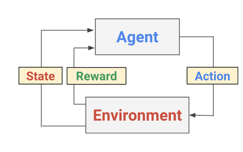
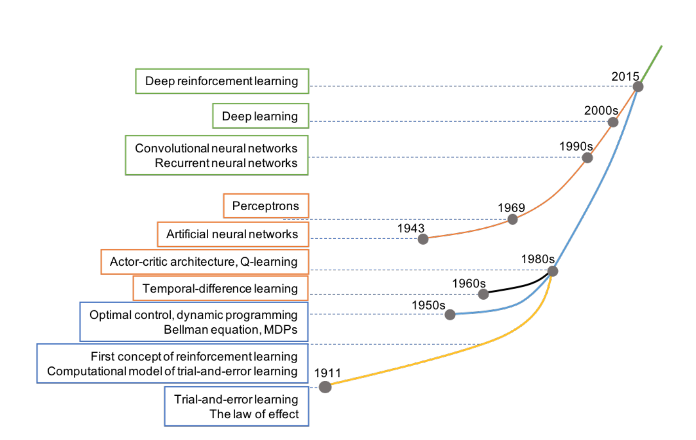

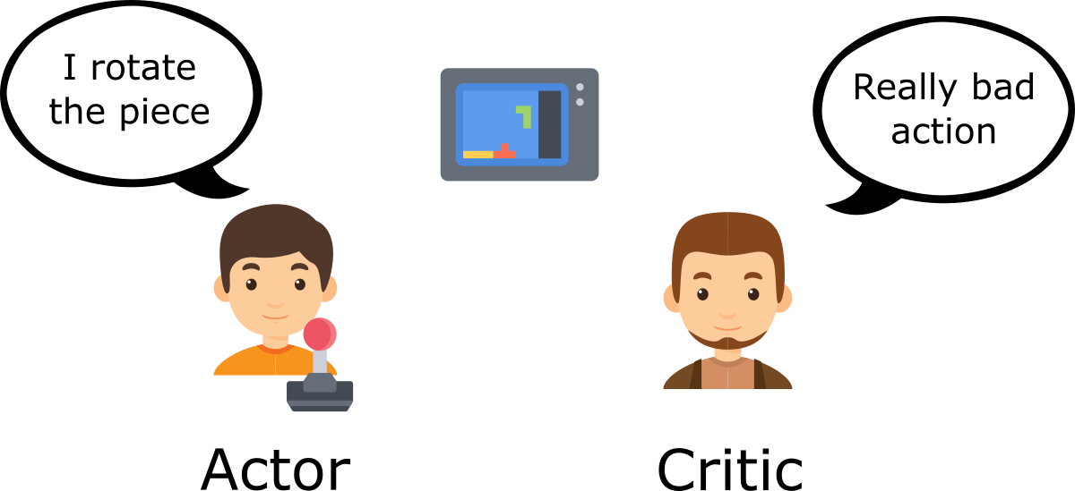
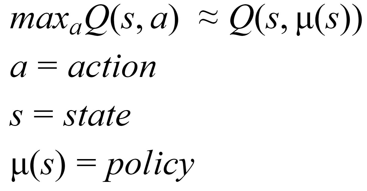
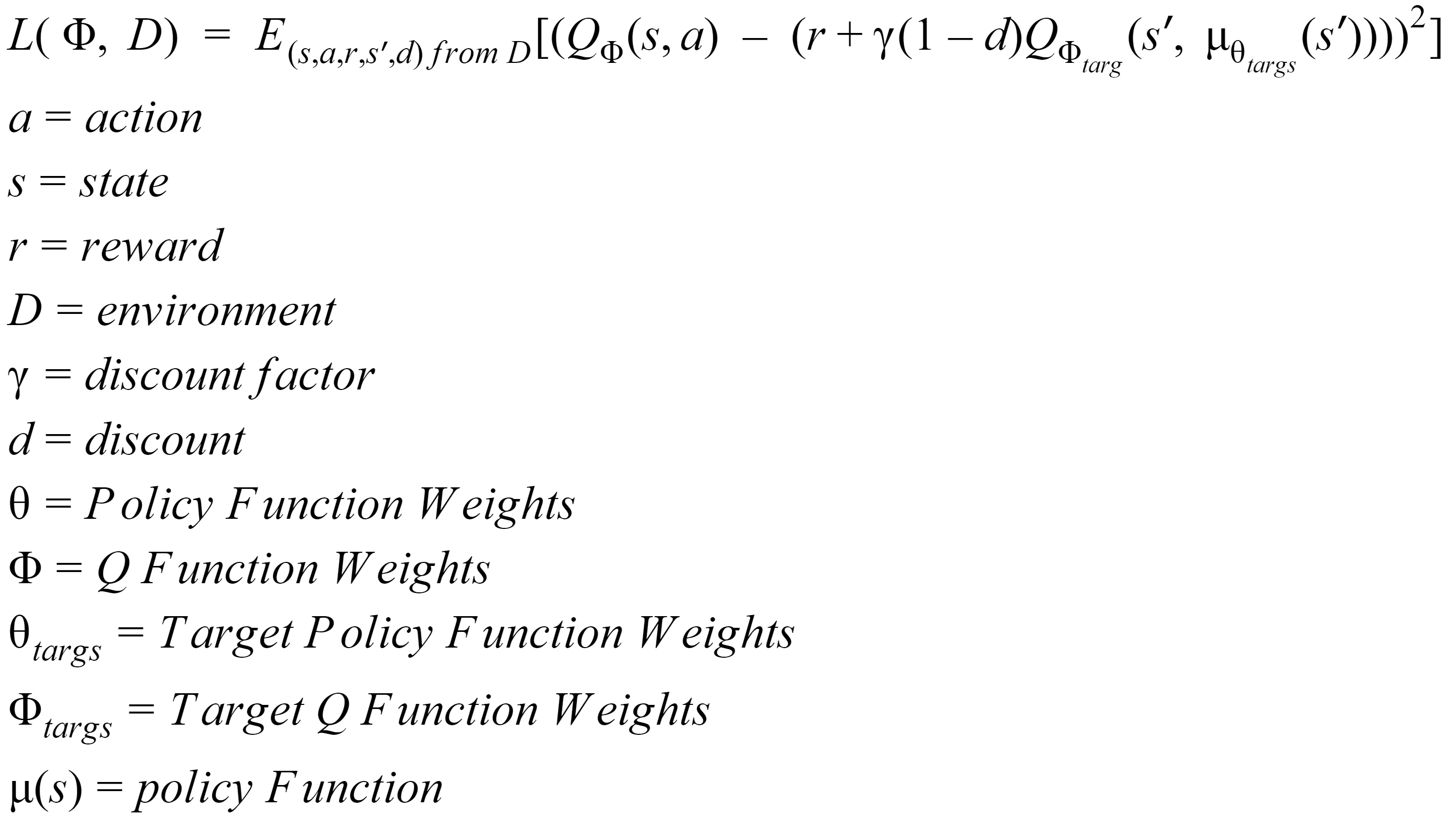
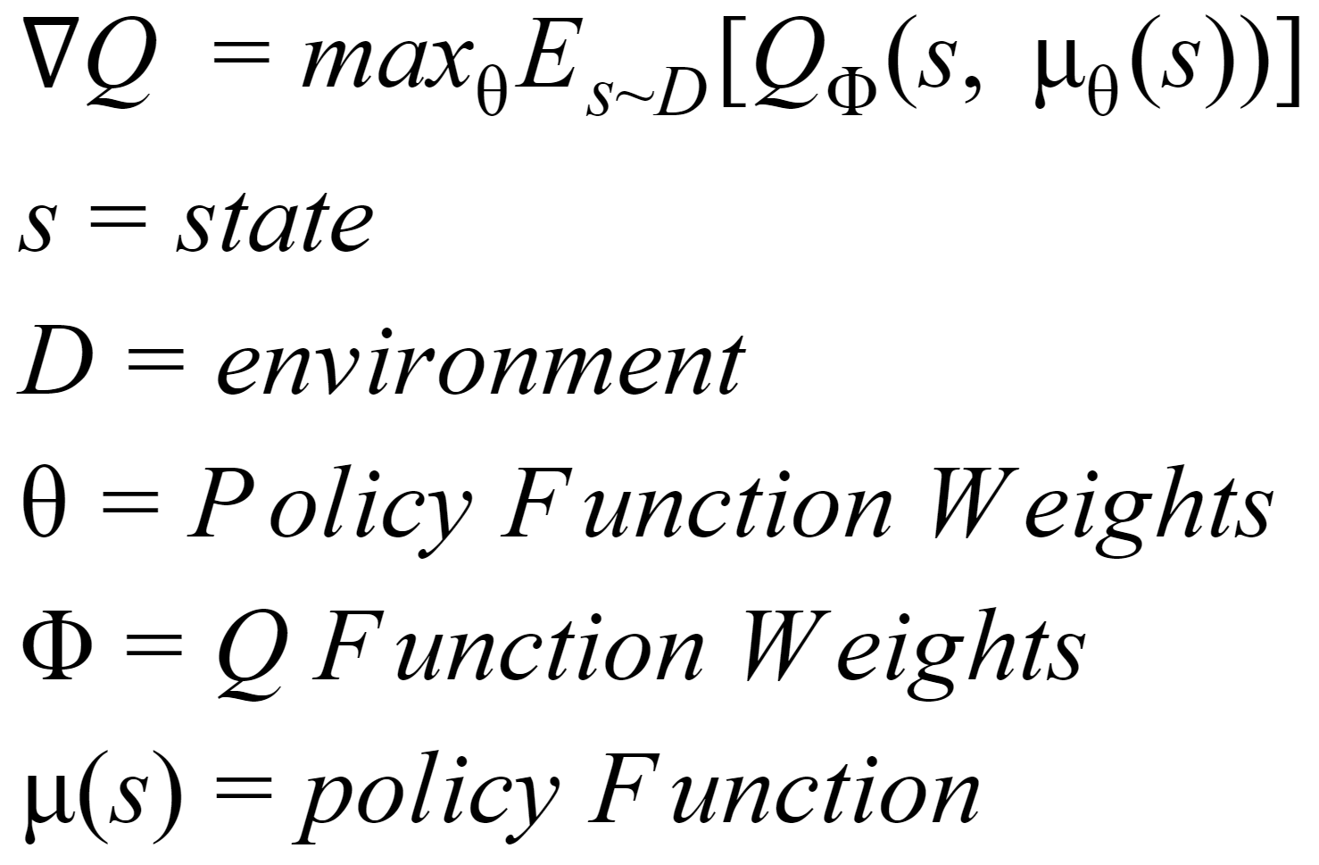
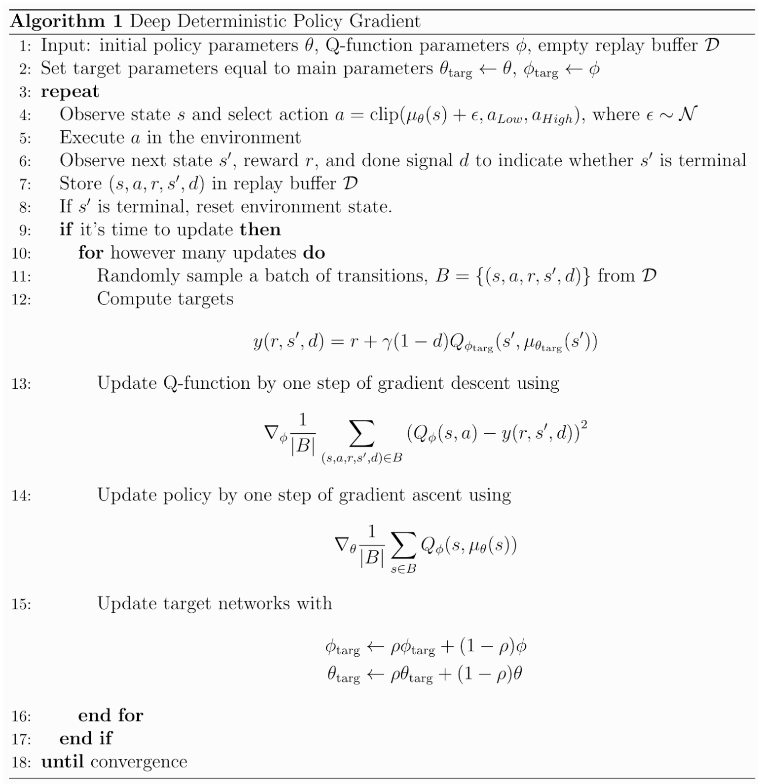
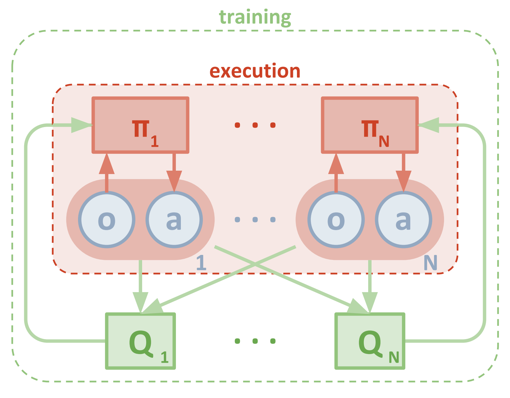 Fig: A prototype of centralized training with decentralized execution
 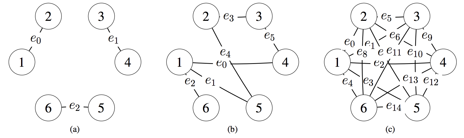 Example coordination graphs for: (a) random partition, (b) overlapping factors, (c) complete factorization
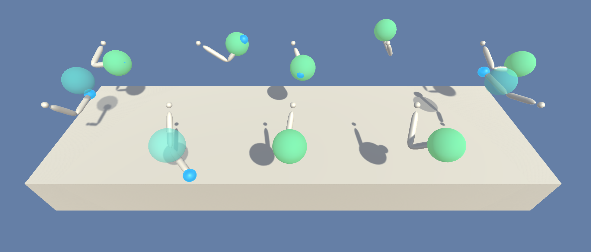

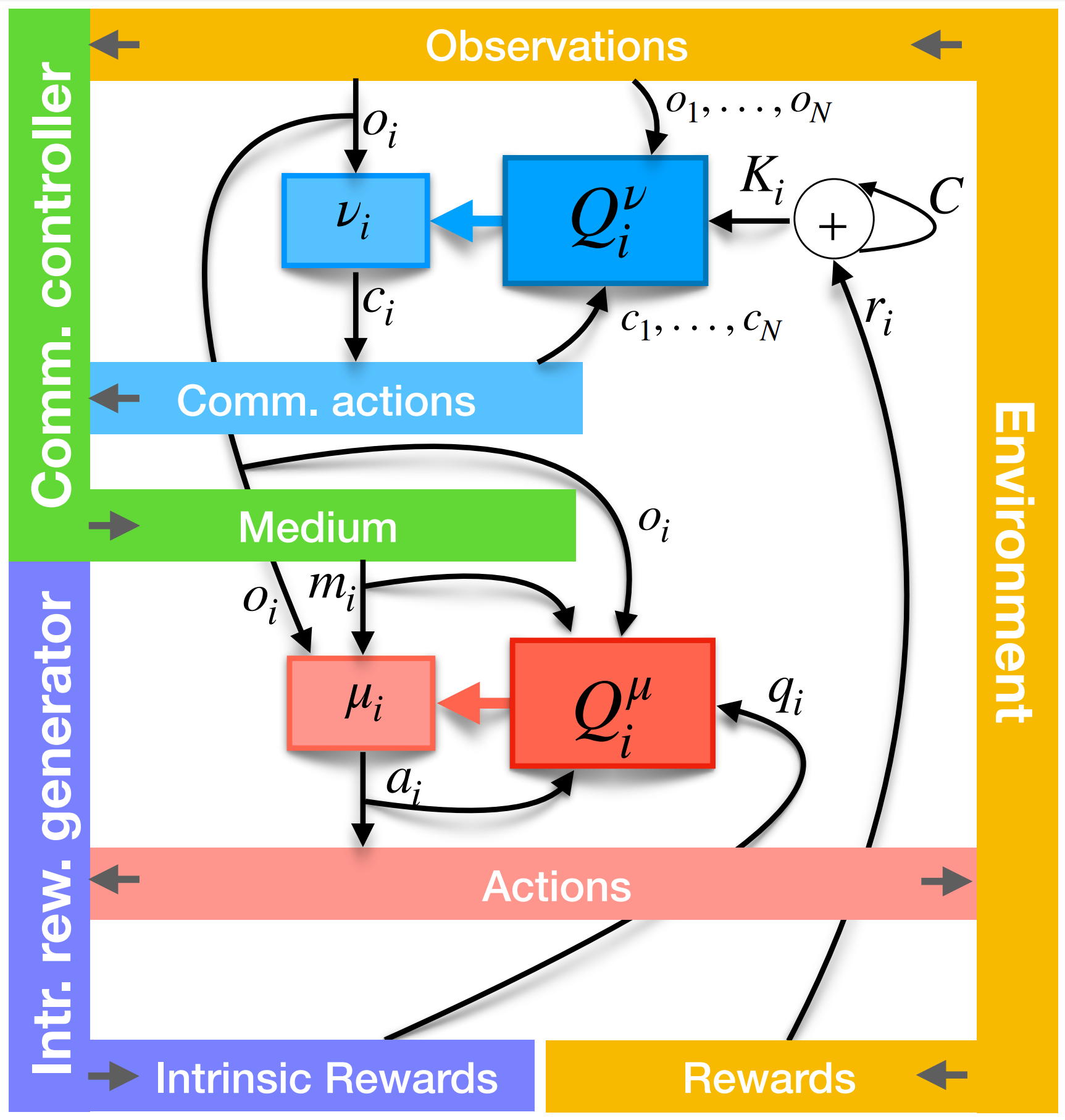
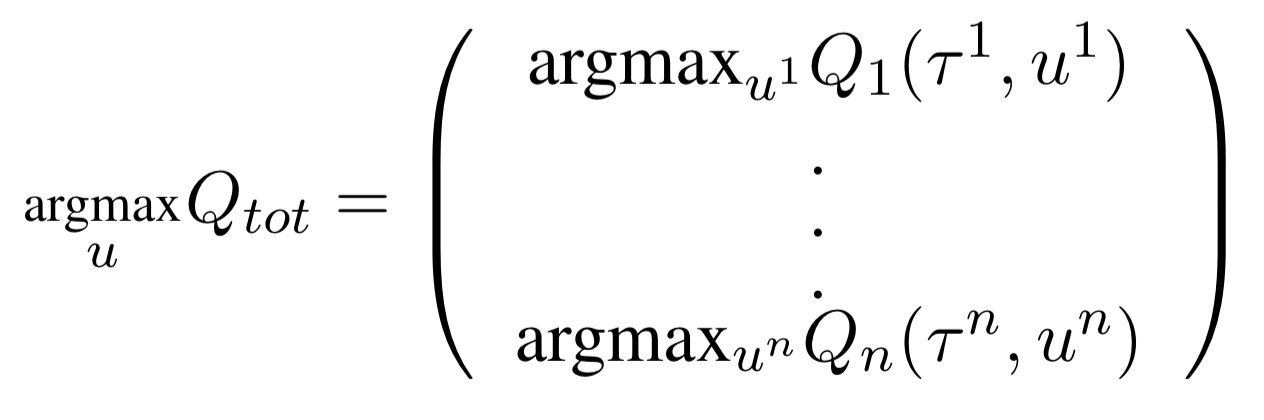
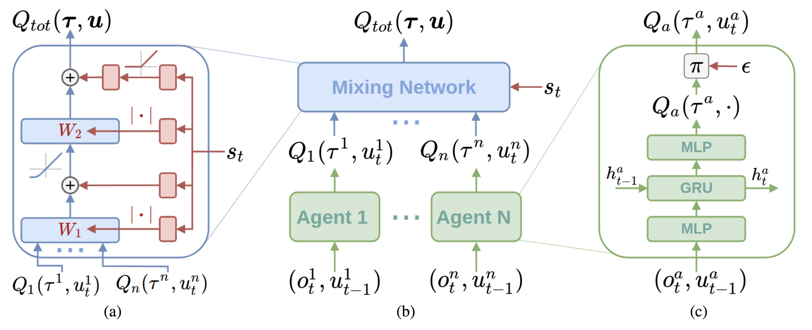 Fig: Qmix architectute taken from
 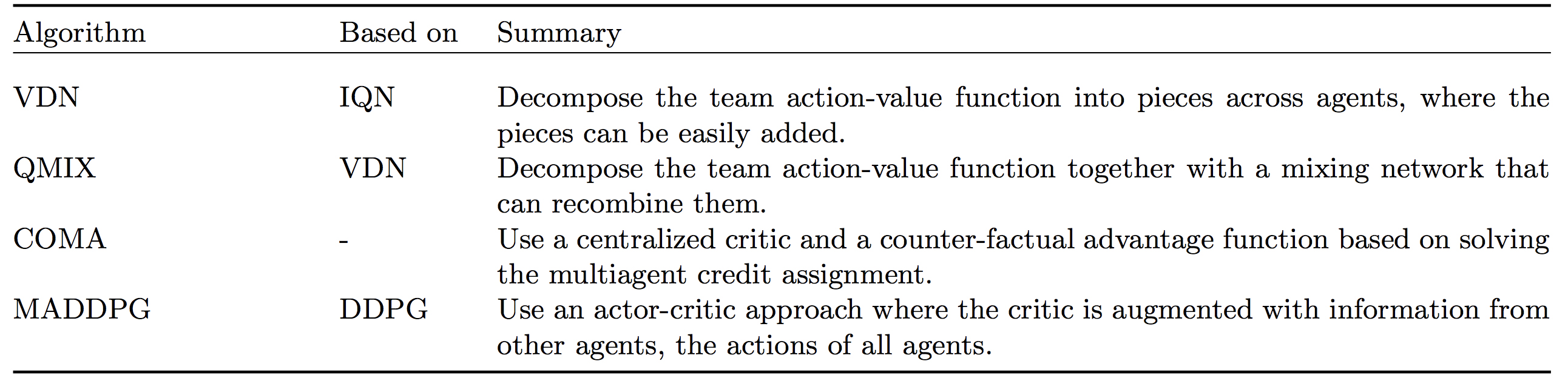 A brief summary of all the approaches taken from the